Linear Ramp Quantum Approximate Optimization Algorithm (LR-QAOA)
Motivation
As quantum processing units (QPUs) surpass the exact classical simulation limit, noise still hinders their practical utility. With increasing qubit counts and circuit depths, there is a pressing need for scalable, interpretable, and platform-agnostic tools that reflect meaningful progress of QPUs performance. The Linear Ramp Quantum Approximate Optimization Algorithm (LR-QAOA) addresses this by offering a deterministic, non-variational QAOA protocol that gives an estimate of the usable circuit depth of a QPU.
Protocol
The LR-QAOA protocol [1] [2] is based on the Quantum Approximate Optimization Algorithm (QAOA), a heuristic designed to find approximate solutions to optimization problems. This protocol uses instances of the Weighted Max Cut (WMC) problem as input. The quality of the solutions found by the quantum computer is assessed using the approximation ratio \(r\), which compares the value of the quantum solution to the optimal (solution of best quality). The QPU is said to pass the test if the sampled solutions’ approximation ratio exceeds that of a random sampler, with a confidence level of \(99.73\%\) (\(\pm 3 \sigma\)). This approach assesses Quantum Processing Units (QPUs) performance at different widths (number of qubits), depths (number of 2-qubit gates), and instance topologies (WMC graph layout).
The key performance metric is the approximation ratio \(r\), which increases with depth and saturates at 1 in the absence of noise, degrading as coherence is lost. LR-QAOA quantifies a QPU’s ability to preserve a coherent signal as circuit depth increases, identifying when performance becomes statistically indistinguishable from random sampling. Currently, the optimal solution is used as the reference for calculating the approximation ratio and is found using the CPLEX solver. To keep the scalability of this protocol, the authors advise using the best-known classical solution if the optimal solution cannot be reached with a classical computer in a reasonable time.
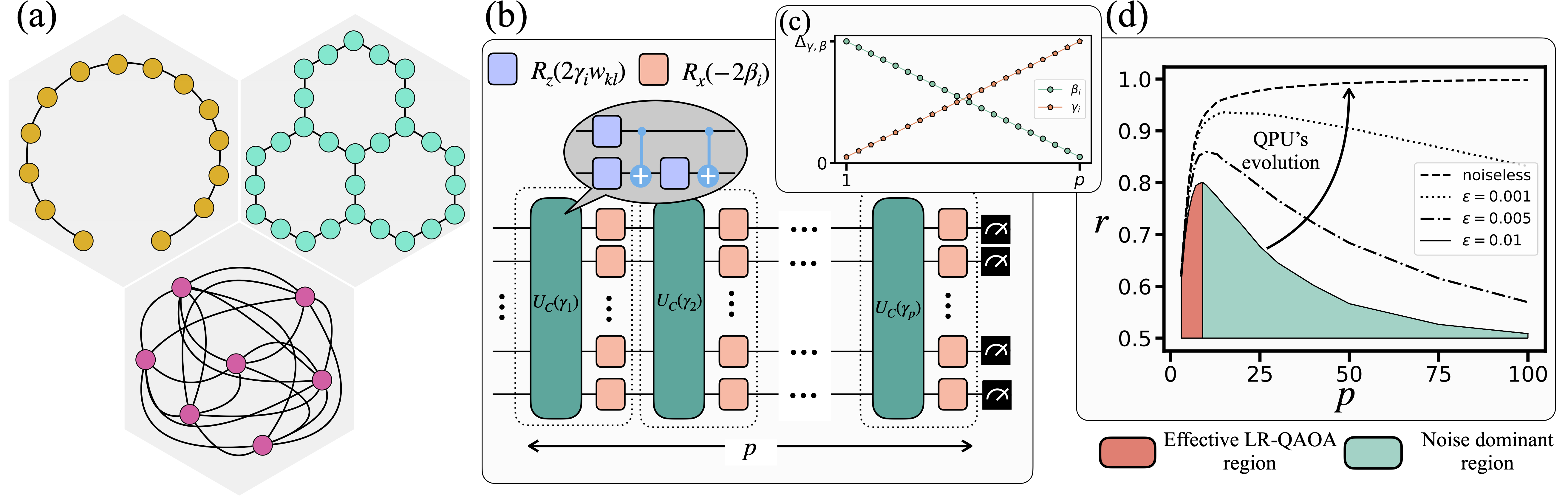
Scheme of the Quantum Processing Units (QPUs) benchmarking. (a) Graphs topologies used for the benchmarking, i.e., the qubit connectivity needed to run the algorithm. In yellow is the 1D-Chain, in green is the native layout (NL), and in pink is the fully connected (FC) graph. (b) QAOA protocol consists of alternating layers of the problem Hamiltonian (green blocks) and the mixer Hamiltonian (pink blocks). \(p\) represents the depth of the algorithm. The parameters \(\gamma_i\) and \(\beta_i\) used in these unitaries follow a linear ramp schedule denoted \(\Delta_{\gamma, \beta}\), as shown in (c). (d) illustrates the typical behavior of the approximation ratio \(r\) as a function of depth \(p\) under different depolarizing noise levels \(\varepsilon\). The red region corresponds to algorithm-dominated performance, and the green region to noise-dominated behavior. As devices improve, the crossover between these regions is expected to occur at larger \(p\).
Assumptions
The protocol is based on well-conditioned ramp schedules with observable signal growth in noise-free settings. For 1D-chain and native layout problems, a fixed ramp value of \(\Delta_{\gamma,\beta} = 1\) is used. For fully connected problems, the value of \(\Delta_{\gamma,\beta}\) depends on the problem size. Experiments done with the same fixed qubit layout and number of qubits share the same parameter \(\Delta_{\gamma,\beta}\) across all tested QPUs (values can be consulted in Table III of [2]).
Rather than setting the optimal values for \(\Delta_{\gamma,\beta}\), this method deterministically fixes these parameters, facilitating replication, scalability, and comparison across different platforms.
Extra pre- and post-processings, such as advanced compilation methods (for fully connected instances, the SWAP strategy employed is detailed in Appendix 7 of [2]), error mitigation, or local search algorithms, are not used in this protocol, as the objective is to capture the raw performance of the QPU.
Limitations
Two limitations have been identified by the authors of [2]:
- The results obtained in the native layout setting must be considered with caution. Indeed, the results obtained from one experiment cannot be directly compared to another if they use a different number of qubits or a different quantum chip topology.
- Another limitation is the difficulty of extrapolating results obtained with this protocol to predict the performance of quantum computers on other applications.
Implementations
The implementation of the experimental setup can be found Here.
Results
This protocol has been used to benchmark 24 QPUs from 6 vendors in [2] for three different kinds of topologies. The results can be found here.
An up-to-date and living version of the benchmarking results is available here. The following sections present the results available in the article [2].
1D-Chain
The 1D-chain benchmark evaluates how well a QPU preserves the algorithmic signal as LR-QAOA depth increases along a linear qubit chain. This topology isolates the impact of circuit depth from layout constraints.
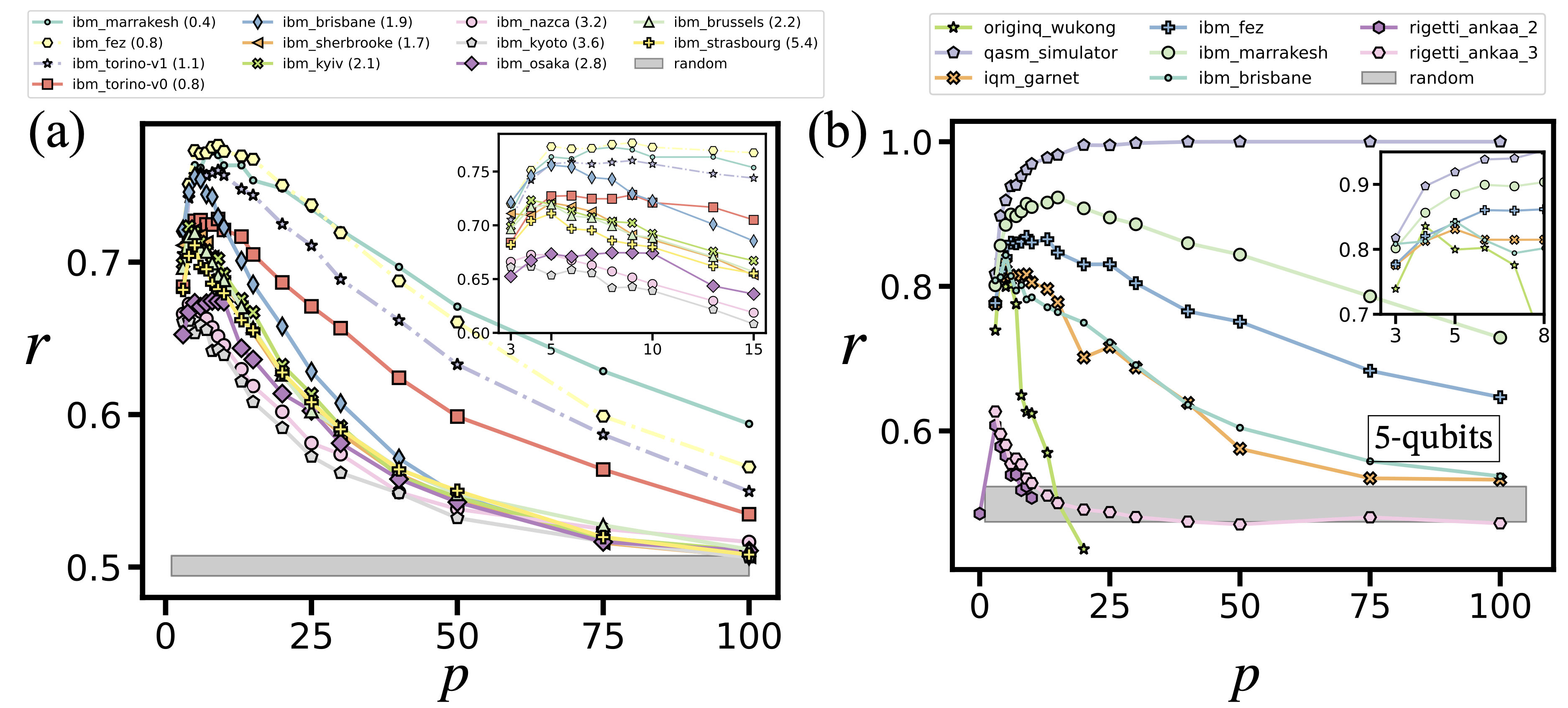
Approximation ratio versus number of LR-QAOA layers for 1D-chain WMC problems on IBM, IQM, Rigetti, and OriginQ devices. (a) Performance on a 100-qubit problem across IBM Eagle and Heron QPUs. Numbers in parentheses indicate Error Per Layered Gate (EPLG) score at the time of execution. (b) Cross-platform comparison for a 5-qubit problem run on different superconducting QPUs.
Native Layout (NL)
The NL benchmark stresses system-wide performance by employing all qubits and native couplers in each device’s layout (it entails that a fair comparison should consider QPUs with a similar number of qubits and a similar layout). Among all tested platforms, only rigetti_ankaa_3 fails to pass the benchmark at any depth. The best-performing devices are ibm_fez, ibm_marrakesh, and ibm_torino, all of which support fractional gates [3] (method to reduce gate count when the circuit only contains single and two-qubit rotations). Interestingly, ibm_aachen achieves a comparable performance peak despite lacking fractional gate support, implying that it could outperform other devices once fractional gates become available on this QPU.
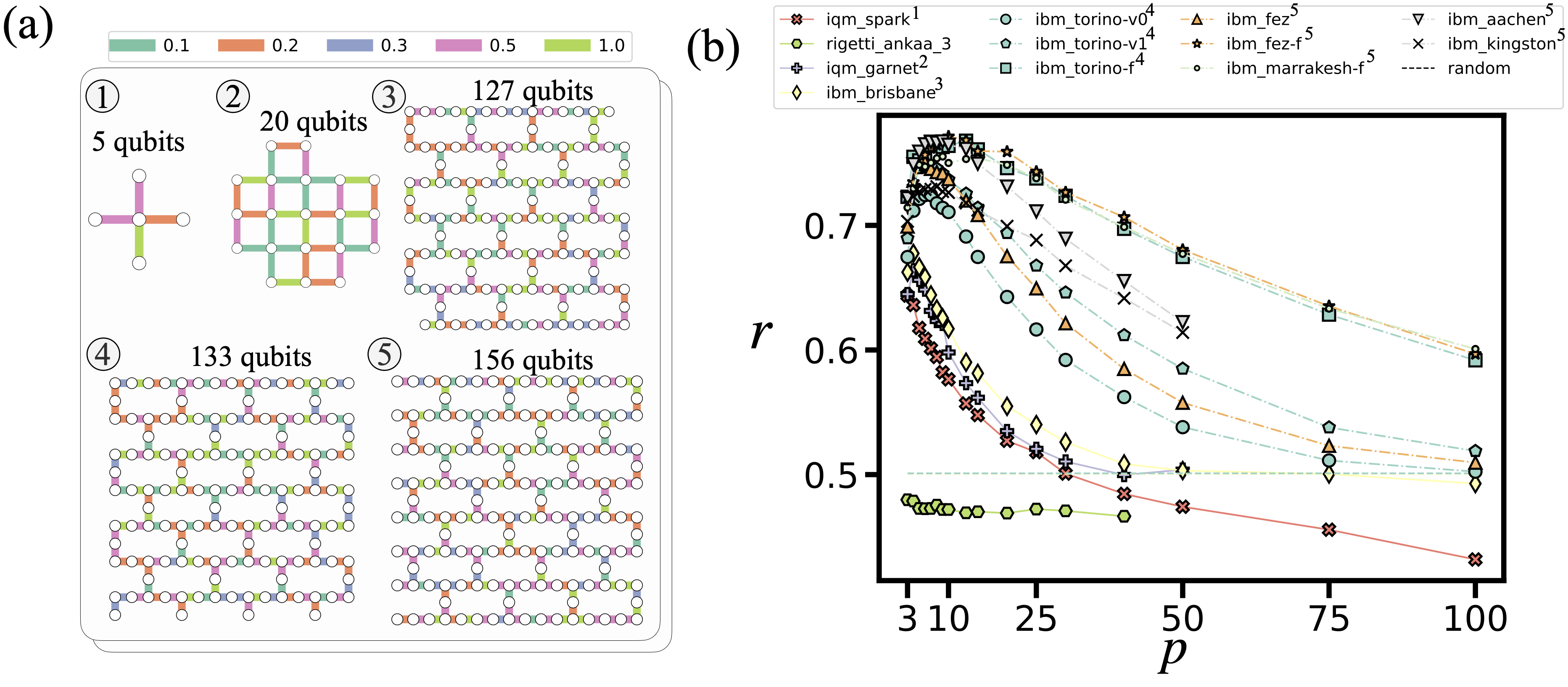
NL-based benchmarking using LR-QAOA for WMC problems on iqm_spark, iqm_garnet, rigetti_ankaa_3, ibm_brisbane, ibm_torino, and ibm_fez/ibm_marrakesh/ibm_aachen/ibm_kingston. Problem sizes (with number of edges in parentheses) are: 5 (4), 20 (30), 82 (138), 127 (144), 133 (150), and 156 (176). (a) QPU layouts used in each experiment. Nodes represent qubits, and edges represent native two-qubit connectivity. Edge colors denote the WMC instance weights, randomly chosen from \(\{0.1, 0.2, 0.3, 0.5, 1\}\), as shown at the top. (b) Approximation ratio versus number of LR-QAOA layers \(p\) for each processor. The dashed horizontal line indicates the random-sampler baseline. Labels with an ‘f’ suffix, e.g., ibm_marrakesh-f, denote experiments using fractional gates.
Fully Connected (FC)
The FC benchmark imposes the highest stress by combining maximal depth and full-qubit connectivity, making it the toughest test of QPU coherence and routing capabilities. Since the approximation ratio achieved by random guessing increases with problem size, the results presented are normalization of the approximation ratio to quantify the gain over random guessing, and denote this normalized metric as \(r_{\text{eff}}\) (see Appendix 3 in [2]).
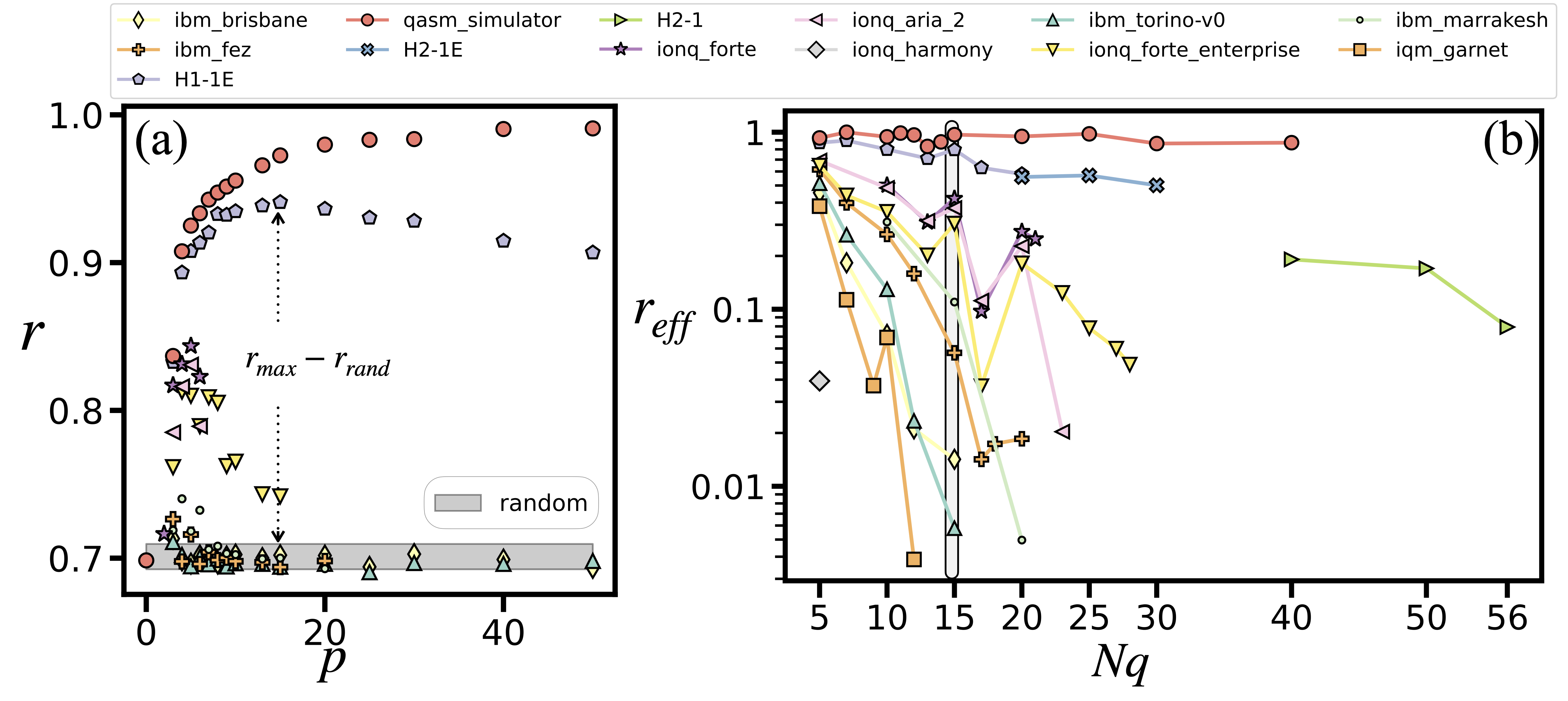
Fully connected (FC) benchmarking using LR-QAOA for WMC problems with 5 to 56 qubits. (a) Approximation ratio \(r\) versus LR-QAOA depth \(p\) for a 15-qubit instance. Shaded region denotes the \(99.73\%\) confidence interval of a random sampler. (b) Effective approximation ratio \(r_{\text{eff}}\) versus problem size for multiple QPUs. Each point reflects the best-performing depth not within the random region.
Performance Summary
The table below summarizes the results of different QPUs; it uses the maximum approximation ratio achieved by each QPU across the three benchmark classes. For the 1D-chain column, the two values correspond to 5- and 100-qubit instances, respectively. Values prefixed with ‘f’ indicate experiments executed using fractional gates. The last column represents the maximum \(N_q\) for which a successful experiment is achieved.
| QPU | 1D-Chain | NL | $$FC_{N_q}=20$$ | $$FC_{N_q}/r_\text{eff}$$ |
|---|---|---|---|---|
| ibm_brisbane | 0.84/0.756 | 0.678 | 0.000 | 16/0.009 |
| ibm_sherbrooke | -/0.721 | 0.664 | - | - |
| ibm_kyiv | -/0.723 | 0.706 | - | - |
| ibm_nazca | -/0.673 | 0.619 | - | - |
| ibm_kyoto | -/0.662 | 0.636 | - | - |
| ibm_osaka | -/0.674 | 0.617 | - | - |
| ibm_brussels | -/0.719 | 0.643 | - | - |
| ibm_strasbourg | -/0.711 | 0.628 | - | - |
| ibm_torino-v0 | -/0.728 | 0.724 | 0.000 | 15/0.006 |
| ibm_torino-v1 | -/0.760 | 0.746, f0.773 | - | - |
| ibm_fez | 0.87/0.776, -/f0.808 | 0.751, f0.782 | 0.020 | 20/0.020 |
| ibm_marrakesh | 0.92/0.773 | f0.772 | 0.004 | 20/0.004 |
| ibm_aachen | - | 0.767 | - | - |
| ibm_kingston | - | 0.731 | - | - |
| H1-1E | - | - | 0.582 | 20/0.582 |
| quantinuum_H2-1 | - | - | 0.555 | 56/0.082 |
| ionq_aria_2 | - | - | 0.227 | 23/0.020 |
| ionq_forte | - | - | 0.269 | 21/0.250 |
| ionq_forte_enterp | - | - | 0.182 | 28/0.049 |
| iqm_spark | - | 0.643 | - | - |
| iqm_garnet | 0.83/- | 0.664 | - | 12/0.004 |
| rigetti_ankaa_2 | 0.61/- | - | - | - |
| rigetti_ankaa_3 | 0.63/- | - | - | - |
| originq_wukong | 0.84/- | - | - | - |
References
- [1]J. A. Montanez-Barrera and K. Michielsen, “Towards a universal QAOA protocol: Evidence of a scaling advantage in solving some combinatorial optimization problems.” 2024.
- [2]J. A. Montanez-Barrera, K. Michielsen, and D. E. B. Neira, “Evaluating the performance of quantum processing units at large width and depth.” 2025.
- [3]IBM, “New fractional gates reduce circuit depth for utility-scale workloads.” Available at: https://www.ibm.com/quantum/blog/fractional-gates