Quantum Process Tomography (QPT)

Motivation

Quantum Process Tomography (QPT) has been proposed to extend quantum state tomography to infer the accuracy of quantum processes [1]. Quantum process tomography aims to precisely reconstruct the linear maps that transform one density matrix representing a quantum state into another. This linear map can be used to characterize the action of quantum gates on qubits precisely.

Protocol

One convenient way to fully qualify the action of quantum processes on quantum states is to expand the density matrix of a quantum state \(\rho\) to a \(4^n\) vector representing the quantum state with respect to an orthogonal Pauli basis. For example, for a 2-qubit state, an orthogonal Pauli basis constructed from the Pauli operators is:

A state \(\rho\) can then be expressed as a linear combination of these operators as:

with \(\alpha_{\{I, X, Y, Z\}^{\otimes n}} \in \mathbb{R}\) and \(\rho_\mathrm{Pauli} \in \mathbb{R}^{4^n}\). For example, if the qubit is initialized in the state \(\rho = \ket{00} \bra{00}\) then it is possible to represent this state as a linear combination of operators that define the orthogonal Pauli basis:

The vector \(\rho_\mathrm{Pauli}\) is then equal to:

The reconstruction of the linear map corresponding to a quantum process (Pauli transfer matrix) is obtained by applying the process to different initial states and measuring them with different observables. Considering the Pauli operators \(\mathcal{P} = \{I, X, Y, Z\}\), the PTM associated with a quantum process on \(n\) qubits is fully characterized by its \(4^n \times 4^n\) different parameters with the \(4^n\) Pauli-basis operators used for defining the eigenstates used as initial states (before the action of the process) and measuring the output state (after the action of the process). The PTM defines how the Pauli coefficients in the vector \(\rho_\mathrm{Pauli}\) evolve with time and it describes how the Pauli components of a quantum state transform under the quantum process.

The following figures are taken from [2]. The left figure represents the Pauli Transfer Matrix (PTM) experimentally measured for the iToffoli gate \(\mathcal{E}_\mathrm{exp}\). The figure on the right shows the difference between the ideal PTM of the iToffoli gate and the actual implementation \(\mathcal{E}_\mathrm{ideal} - \mathcal{E}_\mathrm{exp}\). The procedure for computing the value of a single pixel of the PTM is described after the figure (with an example for the green pixel).

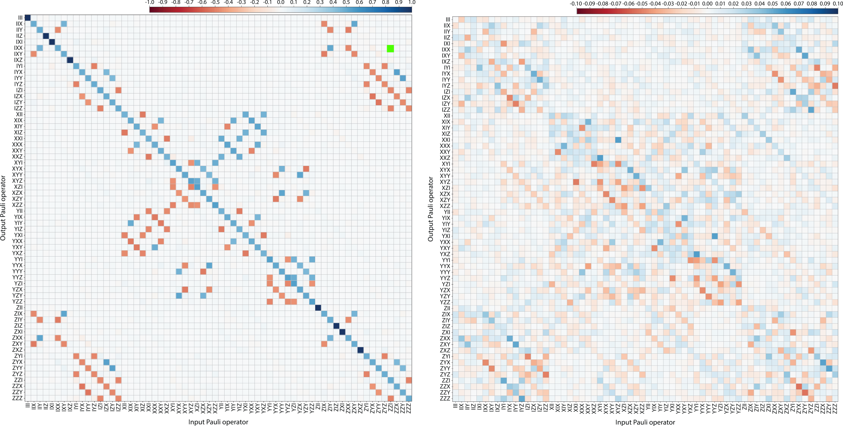
The procedure to compute a value of an intersection in the heatmap (for example the green pixel on the left figure) consists of:

• Preparing the list of eigenstates corresponding to the input operator. For example, if we consider the input operator ZZI (x-axis of the upper figure), the list of considered eigenstates is: \(\ket{000}\) (+1 eigenvalue), \(\ket{010}\) (-1 eigenvalue), \(\ket{100}\) (-1 eigenvalue) and \(\ket{110}\) (+1 eigenvalue). In general, if an input Pauli operator has \(k\) non-identity operators, then \(2^k\) distinct input eigenstates are sufficient, corresponding to all possible \(\pm 1\) eigenvalue assignments of the non-identity operators.
• Computing the expectation value of each evolved eigenstate with respect to the output operator. For example, if we consider the output operator IXX (in the y-axis), the evolved state corresponding to the first eigenstate \(\ket{000}\) is denoted \(\ket{\psi_\mathrm{evolved}(000)} = \mathrm{iToffoli} \ket{000}\). The expectation value is then given by \(\left< \psi_\mathrm{evolved}(000) \lvert IXX \rvert \psi_\mathrm{evolved}(000) \right>\).
• Recombining all the expectation values. The expectation values of each evolved state are then recombined according to the eigenvalue of the input state, and rescaled with a factor depending on the number of different eigenstates considered as input (here \(1/4\) because there are 4 different input eigenstates):

When both the ideal \(\mathcal{E}_\mathrm{ideal}\) and experimental \(\mathcal{E}_\mathrm{exp}\) PTM are known, the process fidelity can be computed as:

with \(d=2^n\) the number of dimensions.

Assumptions

Quantum process tomography relies on the same assumptions as quantum state tomography:

• QPT assumes that every experimental run prepares the qubits in the same state, without correlation with the previous run.
• QPT also assumes that the preparation and measurement of the quantum state are error-free.

Limitations

QPT is time-consuming, and the number of simulations required scales exponentially with the number of qubits involved in the quantum process. For example, evaluating a single intersection on the PTM for a 3-qubit gate requires a series of runs over the \(2^3\) possible input states in the worst case. Assuming it is done for each of the \(4096\) intersections in the PTM, it requires at least running \(\sim 10^4\) different quantum circuits for a total of \(\sim 10^7\) shots (assuming 1000 shots for each circuit).

Extension

Quantum process tomography has been extended to gate-set tomography, which assumes that the native-state preparation, measurement, and gates are subject to errors.

Implementation

An example of QPT implementation is provided in the Qiskit experiments documentation available here.

References

1. [1]I. L. Chuang and M. A. Nielsen, “Prescription for experimental determination of the dynamics of a quantum black box,” Journal of Modern Optics, vol. 44, no. 11-12, pp. 2455–2467, 1997.
2. [2]Y. Kim et al., “High-fidelity three-qubit i Toffoli gate for fixed-frequency superconducting qubits,” Nature physics, vol. 18, no. 7, pp. 783–788, 2022.